scikit-learn User Guide
Complete illustrated guide to machine learning in Python
Complete Illustrated Analysis
From linear regression to neural networks - the essential ML toolkit explained
Linear Models
Ordinary Least Squares (OLS)
The Objective
OLS minimizes: Σ(yᵢ - ŷᵢ)² = ||y - Xw||²
Closed-Form Solution
w = (XTX)-1XTy
This has a direct solution - no iteration needed! But it can be numerically unstable and doesn't handle multicollinearity well.
from sklearn.linear_model import LinearRegression

# Create and fit model
model = LinearRegression()
model.fit(X_train, y_train)

# Get coefficients
print(f"Coefficients: {model.coef_}")
print(f"Intercept: {model.intercept_}")

# Make predictions
y_pred = model.predict(X_test)
Ridge Regression (L2 Regularization)
The Ridge Objective
Minimize: ||y - Xw||² + α||w||²
Why Regularization?
- Prevents overfitting: Penalizes large weights
- Handles multicollinearity: Stabilizes solution
- Shrinks coefficients: But never to exactly zero
The α Parameter
α = 0: Ordinary least squares. α → ∞: All weights → 0. Use cross-validation to find optimal α.
Lasso Regression (L1 Regularization)
The Lasso Objective
Minimize: (1/2n)||y - Xw||² + α||w||₁
Feature Selection
Unlike Ridge, Lasso can set coefficients exactly to zero. This is automatic feature selection! Great when you believe only a few features matter.
When to Use Lasso vs Ridge
- Lasso: When you expect sparse solutions (few important features)
- Ridge: When many features contribute small amounts
- Elastic Net: Combines both (best of both worlds)
Logistic Regression
The Logistic Function (Sigmoid)
P(y=1|x) = 1 / (1 + e-wTx)
Why "Regression" for Classification?
It regresses the log-odds: log(P/(1-P)) = wTx. The output is transformed into probabilities via sigmoid.
Multiclass: One-vs-Rest or Softmax
- OvR: Train K binary classifiers
- Multinomial (Softmax): Single model, K outputs
from sklearn.linear_model import LogisticRegression

# For binary classification
clf = LogisticRegression(C=1.0, solver='lbfgs')
clf.fit(X_train, y_train)

# Predict probabilities
probs = clf.predict_proba(X_test)

# Predict classes
y_pred = clf.predict(X_test)
| Model | Regularization | Feature Selection | Use Case |
|---|---|---|---|
| LinearRegression | None | No | Baseline, interpretability |
| Ridge | L2 (||w||²) | No | Multicollinearity, many features |
| Lasso | L1 (||w||₁) | Yes | Sparse solutions, feature selection |
| ElasticNet | L1 + L2 | Yes | Best of both worlds |
| LogisticRegression | L1/L2/ElasticNet | With L1 | Classification |
Support Vector Machines
The Core Idea
Find the hyperplane that maximizes the margin between classes. The "support vectors" are the data points closest to this hyperplane - they define the decision boundary.
Why SVMs Excel
- High dimensions: Work well when features > samples
- Kernel trick: Non-linear boundaries without explicit transformation
- Robust: Only support vectors matter, not all data

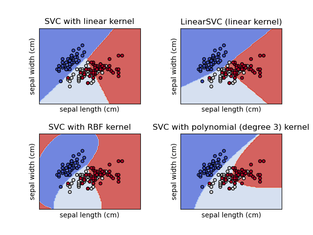
SVC: Support Vector Classification
The C Parameter
C controls the trade-off between smooth decision boundary and classifying training points correctly.
- Small C: Smoother boundary, more misclassifications allowed
- Large C: Harder boundary, fewer misclassifications
Scaling Limitation
O(n²) to O(n³) complexity. For >10K samples, consider LinearSVC or SGDClassifier with hinge loss.
from sklearn.svm import SVC
from sklearn.preprocessing import StandardScaler

# IMPORTANT: Scale your data!
scaler = StandardScaler()
X_train_scaled = scaler.fit_transform(X_train)
X_test_scaled = scaler.transform(X_test)

# RBF kernel (default)
clf = SVC(kernel='rbf', C=1.0, gamma='scale')
clf.fit(X_train_scaled, y_train)
Kernel Functions
Common Kernels
- Linear: K(x,y) = xTy - for linearly separable data
- RBF (Gaussian): K(x,y) = exp(-γ||x-y||²) - most versatile
- Polynomial: K(x,y) = (γxTy + r)d
- Sigmoid: K(x,y) = tanh(γxTy + r)
The RBF Gamma Parameter
γ controls how far the influence of a single training example reaches. Low γ = far reach (smoother), high γ = close reach (more complex).
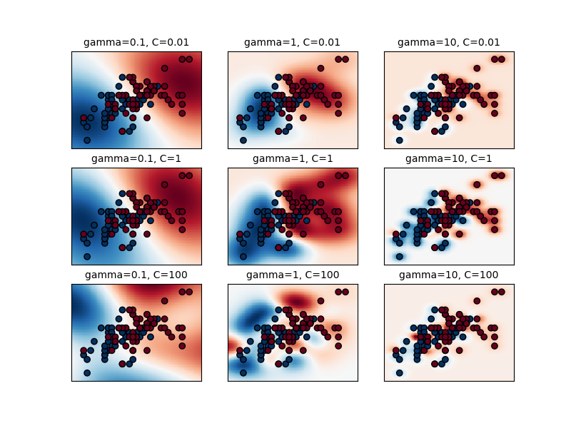
⚠️ Important: Scale Your Data!
SVMs are sensitive to feature scales. Always use StandardScaler or MinMaxScaler before fitting. Without scaling, features with larger values will dominate the kernel computation.
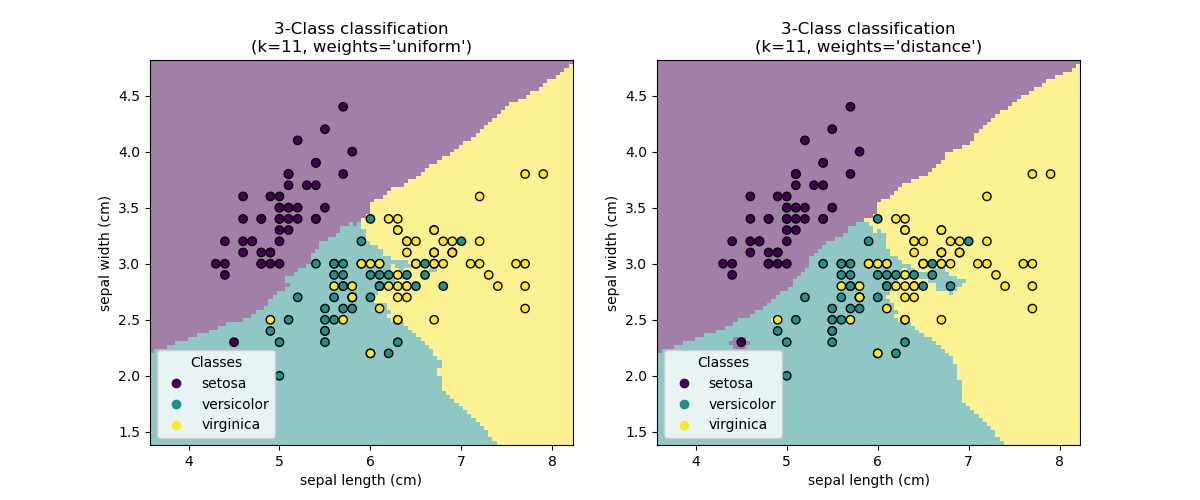
Nearest Neighbors
The Simplest ML Algorithm
KNN is a "lazy learner" - it doesn't build a model, just stores training data. Prediction is: "find k closest points, vote/average their labels."
Advantages
- Simple: No training phase, easy to understand
- Non-parametric: Makes no assumptions about data distribution
- Versatile: Works for classification and regression
Disadvantages
- Slow prediction: Must search all training data
- Memory intensive: Stores all training data
- Curse of dimensionality: Distance becomes meaningless in high dimensions
from sklearn.neighbors import KNeighborsClassifier

# k=5 is a common default
knn = KNeighborsClassifier(n_neighbors=5, weights='uniform')
knn.fit(X_train, y_train)

# Predict
y_pred = knn.predict(X_test)

# Get probabilities (based on neighbor votes)
y_proba = knn.predict_proba(X_test)
KNN Algorithm
- Store all training data
- For a new point x, compute distance to all training points
- Find the k nearest neighbors
- Classification: majority vote of neighbors' labels
- Regression: average (or weighted average) of neighbors' values
When to Use KNN
- Small to medium datasets (< 100K samples)
- Low to medium dimensionality
- When you need a quick baseline
- Recommendation systems (find similar items)
- Anomaly detection (points far from neighbors)
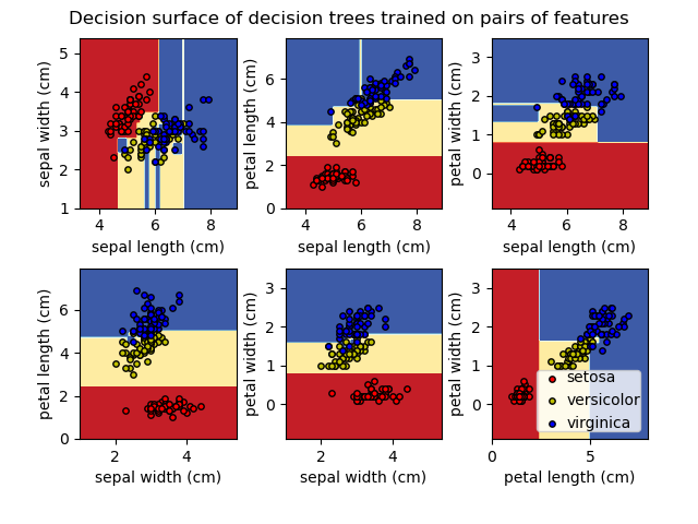
Decision Trees
How Trees Work
A tree recursively splits the data based on feature thresholds. Each internal node is a "question" (e.g., "is feature X > 5?"). Leaves contain predictions.
Key Advantages
- Interpretable: You can visualize and explain the logic
- No scaling needed: Works with raw features
- Handles mixed types: Numerical and categorical
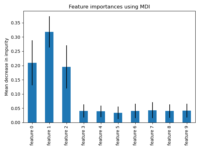
- Feature importance: Built-in feature ranking
Key Disadvantages
- Overfitting: Deep trees memorize training data
- Instability: Small data changes → different trees
- Axis-aligned: Can't capture diagonal boundaries easily
from sklearn.tree import DecisionTreeClassifier, plot_tree
import matplotlib.pyplot as plt

# Create tree with max_depth to prevent overfitting
tree = DecisionTreeClassifier(max_depth=3, random_state=42)
tree.fit(X_train, y_train)

# Visualize the tree
plt.figure(figsize=(20, 10))
plot_tree(tree, feature_names=feature_names,
          class_names=class_names, filled=True)
plt.show()

# Feature importances
print(tree.feature_importances_)
Splitting Criteria
Gini Impurity
Gini = 1 - Σpᵢ² where pᵢ is the probability of class i. Gini = 0 means pure node (all same class).
Entropy
Entropy = -Σpᵢ log(pᵢ). Information gain = parent entropy - weighted child entropy.
In Practice
Gini and entropy usually give similar results. Gini is slightly faster (no log computation).
| Parameter | Purpose | Effect on Overfitting |
|---|---|---|
| max_depth | Maximum tree depth | Lower = less overfitting |
| min_samples_split | Min samples to split a node | Higher = less overfitting |
| min_samples_leaf | Min samples in a leaf | Higher = less overfitting |
| max_features | Features to consider for split | Lower = less overfitting |
| ccp_alpha | Cost-complexity pruning | Higher = more pruning |
Ensemble Methods
Why Ensembles Work
Different models make different errors. By combining them, errors can cancel out. "Wisdom of the crowd" - many weak learners → one strong learner.
Two Main Strategies
- Bagging: Train models independently in parallel, average results (reduces variance)
- Boosting: Train models sequentially, each fixing previous errors (reduces bias)
Random Forest
How Random Forest Works
- Create N bootstrap samples (random sampling with replacement)
- For each sample, train a decision tree
- At each split, consider only √features (random feature subset)
- Aggregate predictions: majority vote (classification) or average (regression)
Why It Works
Bootstrap + random features → decorrelated trees → reduced variance. Individual trees may overfit, but their errors are different and cancel out!
from sklearn.ensemble import RandomForestClassifier

# Create forest with 100 trees
rf = RandomForestClassifier(
    n_estimators=100,      # number of trees
    max_depth=None,        # let trees grow fully
    min_samples_split=2,
    max_features='sqrt',   # √features at each split
    n_jobs=-1,             # use all CPU cores
    random_state=42
)
rf.fit(X_train, y_train)

# Feature importances (averaged across all trees)
importances = rf.feature_importances_
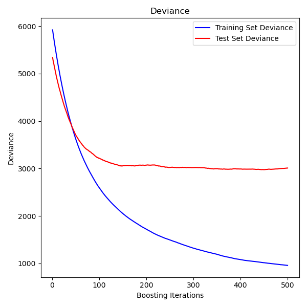
Gradient Boosting
How Gradient Boosting Works
- Start with a simple prediction (e.g., mean)
- Compute residuals (errors)
- Fit a tree to predict the residuals
- Add tree's predictions (scaled by learning rate) to model
- Repeat: fit new trees to new residuals
Key Parameters
- n_estimators: Number of boosting stages
- learning_rate: Shrinks each tree's contribution (lower = more trees needed)
- max_depth: Usually shallow (3-10) for boosting
| Method | Strategy | Trees | Speed | Best For |
|---|---|---|---|---|
| RandomForest | Bagging | Parallel, deep | Fast (parallel) | General purpose, feature importance |
| GradientBoosting | Boosting | Sequential, shallow | Slower | High accuracy, tuned models |
| HistGradientBoosting | Boosting | Sequential, histogram | Very fast | Large datasets, native NaN handling |
| AdaBoost | Boosting | Sequential, stumps | Fast | Simple boosting baseline |
Neural Network Models
When to Use sklearn's Neural Networks
sklearn's MLP is ideal for tabular data where you want neural network benefits without deep learning complexity. It follows the standard fit/predict API, integrates with cross-validation and pipelines, and requires no GPU setup.
Limitations to Consider
- No GPU support: CPU-only, slower for large networks
- Limited architectures: Only fully-connected layers
- No custom layers: Can't build CNNs, RNNs, or transformers
from sklearn.neural_network import MLPClassifier
from sklearn.preprocessing import StandardScaler
from sklearn.pipeline import make_pipeline

# Neural networks REQUIRE scaling!
clf = make_pipeline(
    StandardScaler(),
    MLPClassifier(
        hidden_layer_sizes=(100, 50),  # 2 hidden layers
        activation='relu',            # ReLU activation
        solver='adam',                # Adam optimizer
        max_iter=500,
        early_stopping=True,         # Prevent overfitting
        random_state=42
    )
)

clf.fit(X_train, y_train)
print(f"Accuracy: {clf.score(X_test, y_test):.3f}")
Choosing Architecture Size
- Start small: (100,) often works well
- Add depth: (100, 50) for more complex patterns
- Rule of thumb: Total neurons < training samples
Solver Selection
- adam: Default, works well for most cases
- lbfgs: Better for small datasets (<10k samples)
- sgd: More control, requires tuning learning rate
| Parameter | Options | Default | When to Change |
|---|---|---|---|
| hidden_layer_sizes | tuple of ints | (100,) | Complex data needs more layers |
| activation | relu, tanh, logistic | relu | Rarely - relu works well |
| solver | adam, sgd, lbfgs | adam | lbfgs for small data |
| alpha | float | 0.0001 | Increase for regularization |
| learning_rate_init | float | 0.001 | Lower if not converging |
| early_stopping | bool | False | True to prevent overfitting |
Clustering: Unsupervised Grouping
The Unsupervised Learning Paradigm
Without labels, clustering algorithms use different criteria to define "good" clusters: minimizing within-cluster variance (KMeans), maximizing density (DBSCAN), or building hierarchies (AgglomerativeClustering). The right choice depends on your data's shape and your goals.
Real-World Applications
- Customer segmentation: Group users by behavior
- Anomaly detection: Points far from clusters are outliers
- Data compression: Replace points with cluster centers
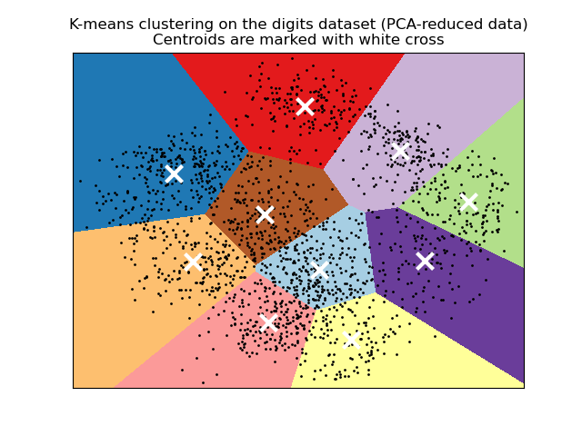
from sklearn.cluster import KMeans
from sklearn.preprocessing import StandardScaler

# Scale features (important for distance-based methods)
X_scaled = StandardScaler().fit_transform(X)

# Fit KMeans with 5 clusters
kmeans = KMeans(n_clusters=5, random_state=42, n_init=10)
labels = kmeans.fit_predict(X_scaled)

# Cluster centers and inertia
centers = kmeans.cluster_centers_
inertia = kmeans.inertia_  # Sum of squared distances to centers
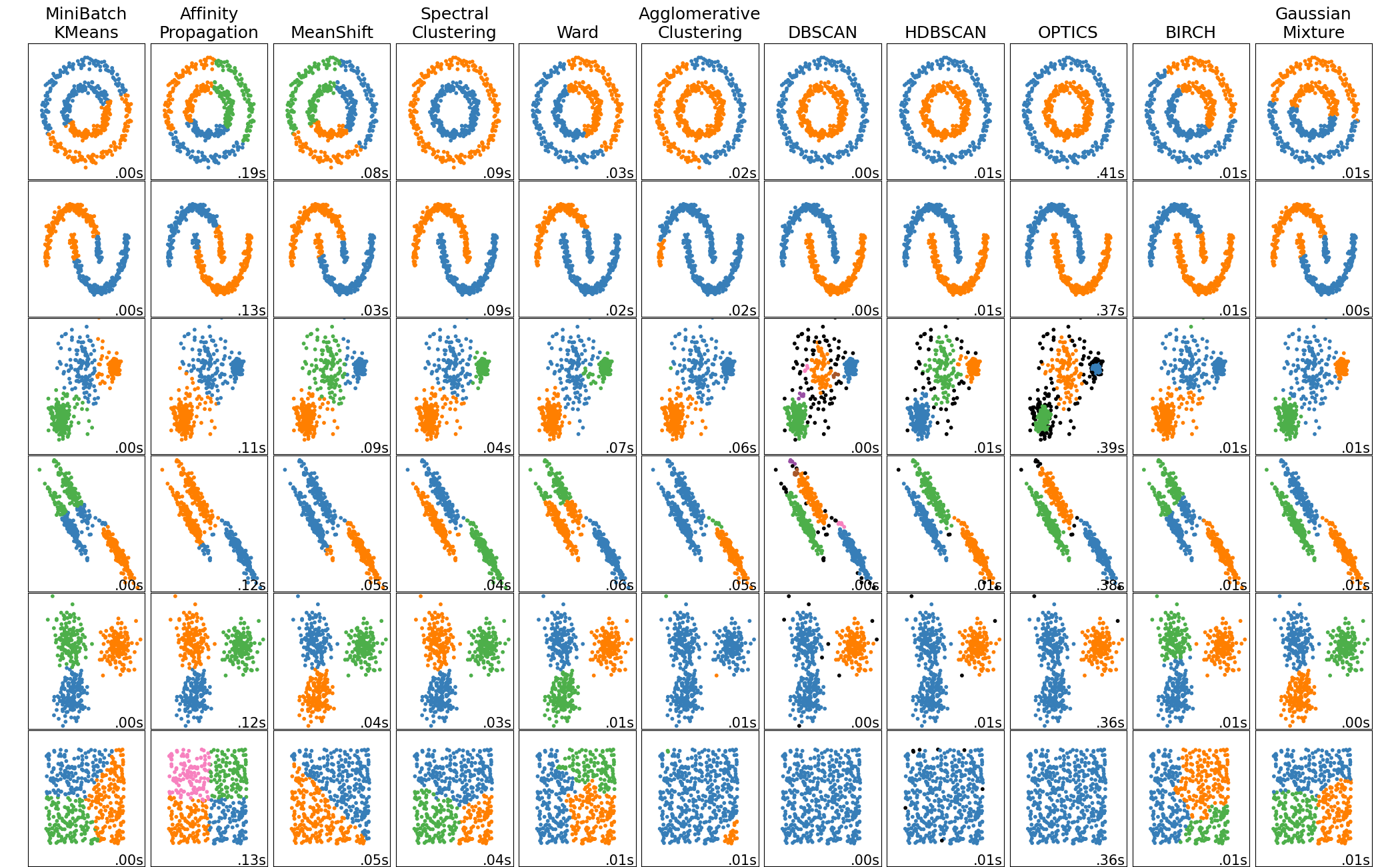
Choosing the Right Algorithm
- KMeans: Fast, spherical clusters, need to know K
- DBSCAN: Arbitrary shapes, handles outliers, no K needed
- Agglomerative: Hierarchical view, works with any linkage
- MiniBatchKMeans: Very large datasets
The K Selection Problem
For KMeans, use the elbow method (plot inertia vs K) or silhouette scores. DBSCAN avoids this but requires tuning eps (neighborhood radius) and min_samples.
from sklearn.cluster import DBSCAN

# eps: max distance between neighbors
# min_samples: minimum points to form a cluster
dbscan = DBSCAN(eps=0.5, min_samples=5)
labels = dbscan.fit_predict(X_scaled)

# -1 labels indicate noise/outliers
n_clusters = len(set(labels)) - (1 if -1 in labels else 0)
n_outliers = list(labels).count(-1)
print(f"Found {n_clusters} clusters, {n_outliers} outliers")
| Algorithm | Cluster Shape | Scalability | Requires K? | Handles Outliers? |
|---|---|---|---|---|
| KMeans | Spherical | O(n) | Yes | No |
| MiniBatchKMeans | Spherical | Very fast | Yes | No |
| DBSCAN | Arbitrary | O(n²) or O(n log n) | No | Yes |
| AgglomerativeClustering | Depends on linkage | O(n²) | Yes | No |
| HDBSCAN | Arbitrary | O(n log n) | No | Yes |
Dimensionality Reduction
Why Reduce Dimensions?
- Curse of dimensionality: Many algorithms degrade with high dimensions
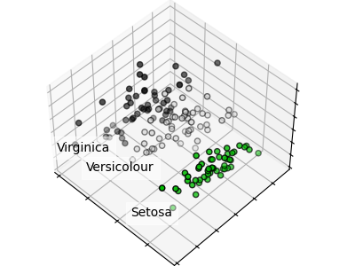
- Visualization: Project to 2D/3D for human understanding
- Noise reduction: Remove low-variance (noisy) components
- Speed: Faster training with fewer features
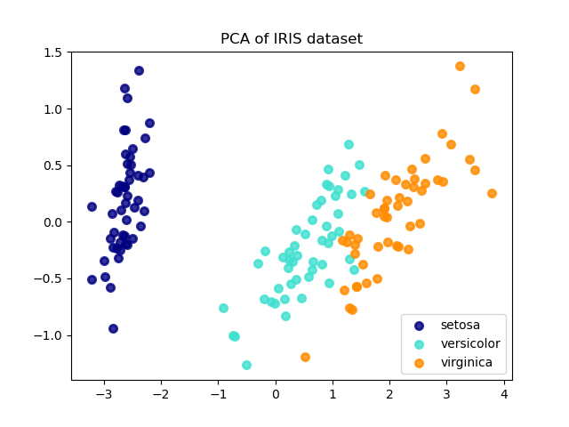
PCA Intuition
PCA finds new axes (principal components) aligned with the directions of maximum variance. The first component captures the most variance, the second captures the most remaining variance orthogonal to the first, and so on.
from sklearn.decomposition import PCA
from sklearn.preprocessing import StandardScaler

# Always standardize before PCA
scaler = StandardScaler()
X_scaled = scaler.fit_transform(X)

# Keep components explaining 95% variance
pca = PCA(n_components=0.95)
X_reduced = pca.fit_transform(X_scaled)

print(f"Reduced: {X.shape[1]} → {X_reduced.shape[1]} features")
print(f"Variance explained: {pca.explained_variance_ratio_.sum():.1%}")
Choosing the Right Method
- PCA: General purpose, linear, unsupervised
- TruncatedSVD: Sparse data (text, counts)
- LDA: When you have labels and want class separation
- t-SNE: Visualization only (slow, non-deterministic)
How Many Components?
Use n_components=0.95 to keep 95% variance, or plot cumulative explained variance ratio to find the "elbow". For visualization, use n_components=2 or 3.
from sklearn.pipeline import Pipeline
from sklearn.decomposition import PCA
from sklearn.linear_model import LogisticRegression

# PCA as preprocessing in a pipeline
pipe = Pipeline([
    ('scaler', StandardScaler()),
    ('pca', PCA(n_components=50)),
    ('clf', LogisticRegression())
])

# Tune n_components with GridSearchCV
from sklearn.model_selection import GridSearchCV
param_grid = {'pca__n_components': [10, 30, 50, 100]}
search = GridSearchCV(pipe, param_grid, cv=5)
search.fit(X_train, y_train)
| Method | Type | Supervised? | Best For |
|---|---|---|---|
| PCA | Linear | No | General preprocessing, variance preservation |
| TruncatedSVD | Linear | No | Sparse matrices, text data (LSA) |
| LDA | Linear | Yes | Classification preprocessing |
| t-SNE | Nonlinear | No | Visualization only |
| UMAP | Nonlinear | No | Visualization, faster than t-SNE |
| NMF | Linear | No | Non-negative data (images, text) |
Cross-Validation and Model Selection
Why Cross-Validation Matters
A single train/test split can be lucky or unlucky. Cross-validation averages over multiple splits, giving you both a mean score and standard deviation. This helps detect if your model's performance varies wildly across different data subsets.
Common CV Strategies
- KFold: Standard K splits, default K=5
- StratifiedKFold: Preserves class proportions (classification)
- LeaveOneOut: K = n, expensive but unbiased
- TimeSeriesSplit: Respects temporal order
from sklearn.model_selection import cross_val_score, cross_validate
from sklearn.ensemble import RandomForestClassifier

clf = RandomForestClassifier(n_estimators=100)

# Simple: Get array of scores
scores = cross_val_score(clf, X, y, cv=5, scoring='accuracy')
print(f"Accuracy: {scores.mean():.3f} (+/- {scores.std()*2:.3f})")

# Detailed: Multiple metrics, timing
results = cross_validate(clf, X, y, cv=5,
    scoring=['accuracy', 'f1_macro'],
    return_train_score=True
)
print(results['test_accuracy'])
print(results['fit_time'])
Grid vs Random Search
- GridSearchCV: Tests all combinations. Good for small grids.
- RandomizedSearchCV: Samples n_iter combinations. Better for large spaces.
- Research shows: 60 random iterations often beats exhaustive grid search
Avoiding Data Leakage
Always put preprocessing inside the cross-validation loop. Use Pipeline to ensure scaling/encoding is fit only on training folds, not the entire dataset.
from sklearn.model_selection import GridSearchCV
from sklearn.pipeline import Pipeline
from sklearn.svm import SVC

# Pipeline ensures no data leakage
pipe = Pipeline([
    ('scaler', StandardScaler()),
    ('svc', SVC())
])

# Parameter grid (use double underscore for nested params)
param_grid = {
    'svc__C': [0.1, 1, 10, 100],
    'svc__kernel': ['rbf', 'linear'],
    'svc__gamma': ['scale', 'auto', 0.1, 0.01]
}

search = GridSearchCV(pipe, param_grid, cv=5, scoring='f1_macro', n_jobs=-1)
search.fit(X_train, y_train)

print(f"Best params: {search.best_params_}")
print(f"Best CV score: {search.best_score_:.3f}")
print(f"Test score: {search.score(X_test, y_test):.3f}")
| Scorer | Task | Best When |
|---|---|---|
| accuracy | Classification | Balanced classes |
| f1, f1_macro, f1_weighted | Classification | Imbalanced classes |
| roc_auc | Binary classification | Ranking quality matters |
| neg_mean_squared_error | Regression | General regression |
| r2 | Regression | Variance explained |
| neg_log_loss | Classification | Probability calibration matters |
Data Preprocessing
Why Preprocessing Matters
- Scaling: Many algorithms (SVM, KNN, neural nets) are sensitive to feature scales
- Encoding: ML models need numeric inputs, not strings
- Missing values: Most algorithms can't handle NaN
Fit vs Transform
Fit learns parameters from training data (mean, std, categories). Transform applies those parameters. Always fit on training data only, then transform both train and test to avoid data leakage.
from sklearn.preprocessing import StandardScaler, MinMaxScaler, RobustScaler

# StandardScaler: zero mean, unit variance (most common)
scaler = StandardScaler()
X_scaled = scaler.fit_transform(X_train)
X_test_scaled = scaler.transform(X_test)  # Use train params!

# MinMaxScaler: scale to [0, 1] range
scaler = MinMaxScaler()

# RobustScaler: use median/IQR, robust to outliers
scaler = RobustScaler()
Encoding Strategy
- Ordinal: Education level (high school < bachelor < master)
- One-Hot: Colors, countries, product categories
- Target encoding: High-cardinality categories (use category_encoders library)
Common Pitfall
Don't use OneHot for high-cardinality features (1000+ categories). This creates sparse matrices and can cause overfitting. Consider target encoding or hashing instead.
from sklearn.preprocessing import OneHotEncoder, StandardScaler
from sklearn.compose import ColumnTransformer
from sklearn.impute import SimpleImputer
from sklearn.pipeline import Pipeline

# Define column groups
numeric_features = ['age', 'income', 'score']
categorical_features = ['gender', 'city', 'category']

# Create preprocessing pipelines for each type
numeric_transformer = Pipeline([
    ('imputer', SimpleImputer(strategy='median')),
    ('scaler', StandardScaler())
])

categorical_transformer = Pipeline([
    ('imputer', SimpleImputer(strategy='constant', fill_value='missing')),
    ('onehot', OneHotEncoder(handle_unknown='ignore'))
])

# Combine with ColumnTransformer
preprocessor = ColumnTransformer([
    ('num', numeric_transformer, numeric_features),
    ('cat', categorical_transformer, categorical_features)
])
| Scaler | Formula | Use When |
|---|---|---|
| StandardScaler | (x - mean) / std | Default choice, assumes Gaussian |
| MinMaxScaler | (x - min) / (max - min) | Bounded features, neural networks |
| RobustScaler | (x - median) / IQR | Data has outliers |
| MaxAbsScaler | x / max(|x|) | Sparse data, preserves zeros |
| Normalizer | x / ||x|| | Per-sample L2 normalization (text) |
Pipelines and Composite Estimators
Why Pipelines Are Essential
- No data leakage: Fit only sees training fold in CV
- Clean code: One object does fit → transform → predict
- Reproducible: Same pipeline produces same results
- Deployable: Pickle the pipeline, deploy anywhere
Pipeline Behavior
When you call pipeline.fit(X, y), it calls fit_transform on all transformers in sequence, then fit on the final estimator. predict() calls transform on all transformers, then predict on the final estimator.
from sklearn.pipeline import Pipeline
from sklearn.compose import ColumnTransformer
from sklearn.preprocessing import StandardScaler, OneHotEncoder
from sklearn.impute import SimpleImputer
from sklearn.ensemble import RandomForestClassifier
from sklearn.model_selection import GridSearchCV

# Feature groups
num_cols = ['age', 'balance']
cat_cols = ['job', 'education']

# Preprocessor
preprocessor = ColumnTransformer([
    ('num', Pipeline([
        ('impute', SimpleImputer(strategy='median')),
        ('scale', StandardScaler())
    ]), num_cols),
    ('cat', Pipeline([
        ('impute', SimpleImputer(strategy='most_frequent')),
        ('encode', OneHotEncoder(handle_unknown='ignore'))
    ]), cat_cols)
])

# Full pipeline
pipe = Pipeline([
    ('preprocess', preprocessor),
    ('classifier', RandomForestClassifier())
])

# GridSearch with nested parameter names
param_grid = {
    'classifier__n_estimators': [100, 200],
    'classifier__max_depth': [10, 20, None]
}

search = GridSearchCV(pipe, param_grid, cv=5, n_jobs=-1)
search.fit(X_train, y_train)
print(f"Best score: {search.best_score_:.3f}")
Pipeline vs FeatureUnion
- Pipeline: Sequential (A → B → C), output of A is input to B
- FeatureUnion: Parallel, same input to A, B, C; outputs concatenated
- ColumnTransformer: Different columns to different transformers
make_pipeline Shortcut
Use make_pipeline(StandardScaler(), PCA(50), LogisticRegression()) for quick pipelines. Step names are auto-generated from class names (lowercase).
import joblib

# Save the fitted pipeline
joblib.dump(pipe, 'model_pipeline.pkl')

# Load for inference
loaded_pipe = joblib.load('model_pipeline.pkl')
predictions = loaded_pipe.predict(new_data)

# The loaded pipeline includes ALL preprocessing
# Just pass raw data - it handles everything
Glossary
Key terms and concepts in scikit-learn
Quick Reference Cheat Sheet
Common patterns and best practices
The Universal API Pattern
from sklearn.module import ModelClass

# 1. Instantiate
model = ModelClass(hyperparameters)

# 2. Fit
model.fit(X_train, y_train)

# 3. Predict
y_pred = model.predict(X_test)

# 4. Evaluate
score = model.score(X_test, y_test)
Common Workflow
from sklearn.model_selection import train_test_split, cross_val_score
from sklearn.preprocessing import StandardScaler
from sklearn.pipeline import Pipeline
from sklearn.ensemble import RandomForestClassifier

# Split data
X_train, X_test, y_train, y_test = train_test_split(
    X, y, test_size=0.2, random_state=42
)

# Create pipeline
pipe = Pipeline([
    ('scaler', StandardScaler()),
    ('clf', RandomForestClassifier())
])

# Cross-validation
scores = cross_val_score(pipe, X_train, y_train, cv=5)
print(f"CV Score: {scores.mean():.3f} (+/- {scores.std():.3f})")

# Final fit and evaluation
pipe.fit(X_train, y_train)
print(f"Test Score: {pipe.score(X_test, y_test):.3f}")
Why Start with Linear Models?
Linear models are interpretable, fast, and often surprisingly effective. They form the basis for understanding more complex models. Even neural networks are stacks of linear transformations with non-linear activations.
Key Advantages